Income elasticity of demand

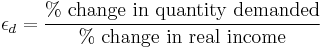
In economics, income elasticity of demand measures the responsiveness of the demand for a good to a change in the income of the people demanding the good, ceteris paribus. It is calculated as the ratio of the percentage change in demand to the percentage change in income. For example, if, in response to a 10% increase in income, the demand for a good increased by 20%, the income elasticity of demand would be 20%/10% = 2.

1 Interpretation
2 Mathematical definition
3 Selected income elasticities
4 See also
5 Notes
6 References

Interpretation

A negative income elasticity of demand is associated with inferior goods; an increase in income will lead to a fall in the demand and may lead to changes to more luxurious substitutes.
A positive income elasticity of demand is associated with normal goods; an increase in income will lead to a rise in demand. If income elasticity of demand of a commodity is less than 1, it is a necessity good. If the elasticity of demand is greater than 1, it is a luxury good or a superior good.
A zero income elasticity (or inelastic) demand occurs when an increase in income is not associated with a change in the demand of a good. These would be sticky goods.

Income elasticity of demand can be used as an indicator of industry health, future consumption patterns and as a guide to firms investment decisions. For example, the "selected income elasticities" below suggest that an increasing portion of consumer's budgets will be devoted to purchasing automobiles and restaurant meals and a smaller share to tobacco and margarine.^[1]

Income elasticities are closely related to the population income distribution and the fraction of a the product's sales attributable to buyers from different income brackets. Specifically when a buyer in a certain income bracket experiences an income increase, their purchase of a product changes to match that of individuals in their new income bracket. If the income share elasticity is defined as the negative percentage change in individuals given a percentage increase in income bracket, then the income-elasticity, after some computation, becomes the expected value of the income-share elasticity with respect to the income distribution of purchasers of the product. When the income distribution is described by a gamma distribution, the income elasticity is proportional to the percentage difference between the average income of the product's buyers and the average income of the population.^[2].

Mathematical definition

$\epsilon_d = \frac{\%\ \mbox{change in quantity demanded}}{\%\ \mbox{change in real income}}$

More formally, the income elasticity of demand, $\ \epsilon_d$ , for a given Marshallian demand function $Q(I,\vec{P})$ for a good is

$\epsilon_d = \frac{\partial Q}{\partial I}\frac{I}{Q}$

or alternatively:

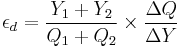
$\epsilon_d={Y_1 %2B Y_2 \over Q_1 %2B Q_2}\times{\Delta Q \over \Delta Y}$

This can be rewritten in the form:

$\epsilon_d = \frac{d \ln Q}{d \ln I}$

With income $I$ , and vector of prices $\vec{P}$ . Many necessities have an income elasticity of demand between zero and one: expenditure on these goods may increase with income, but not as fast as income does, so the proportion of expenditure on these goods falls as income rises. This observation for food is known as Engel's law.

Selected income elasticities

Automobiles 2.46^[3]
Books 1.44
Restaurant Meals 1.40
Tobacco 0.64
Margarine −0.20
Public Transportation −0.36^[4]

Income elasticities are notably stable over time and across countries.^[5]

Notes

^ Frank, Robert (2008). p. 125
^ Bordley and McDonald.
^ Samuelson; Nordhaus (2001). p.94.
^ Frank (2008) 125.
^ Perloff, J. (2008). p.105.

References

Bordley; McDonald. "Estimating Income Elasticities from the Average Income of a Product's Buyers and the Population Income Distribution". Journal of Business and Economic Statistics.
Perloff, J. (2008). Microeconomics Theory & Applications with Calculus. Pearson. ISBN 9780321277947.
Samuelson; Nordhaus (2001). Microeconomics (17th ed.). McGraw-Hill.
Frank, Robert (2008). Microeconomics and Behavior (7th ed.). McGraw-Hill. ISBN 978-007-126349-8.